Score-Based Generative Modeling through Stochastic Differential Equations
https://arxiv.org/pdf/2011.13456
1. Introduction
- Training data에 노이즈를 추가한 후, 그 노이즈를 제거하는 방법을 학습해 뛰어난 성과를 보인 생성 모델을 Score matching with Langevin dynamics(SMLD)와 Denoising diffusion probabilistic modeling(DDPM)에서 다루었다. 여기서, DDPM의 training objective는 각각의 noise scale에 대한 score를 계산하게 되고 이는 두 방법이 같은 방법을 사용한다는 것을 의미한다. 따라서, 두 가지 생성 모델의 방법 모두를 score-based generative model이라고 부르기로 한다.
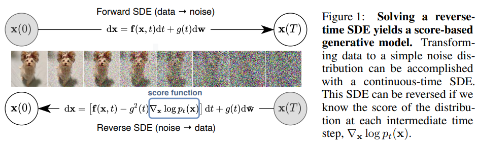
- 유한개의 노이즈 분포에 따라서 데이터에 노이즈를 추가하는 방법 대신에, 연속적인 노이즈 분포를 시간에 따라서 데이터에 추가하기로 한다(노이즈가 확산하는 것과 같아 diffusion이라 부른다). 이 과정에서 데이터 분포가 점진적으로 확산되어 노이즈로 분포가 되고, prescribed SDE의 형태로 나타나게 된다. 이 과정을 reverse해 random noise를 새로운 샘플을 만들어내도록 변형할 수 있다. 이러한 역과정은 reverse-time SDE를 만족하고, forward SDE로 부터 유도될 수 있다. 따라서, reverse-time SDE는 time-dependent neural network를 학습하는 방법을 통해 얻을 수 있고, numerical SDE solvers를 통해 샘플을 만들어낼 수 있게 된다.
- 이와 같은 접근은 다음과 같은 장점을 가진다.
- Flexible sampling and likelihood computation: 일반적인 SDE solver을 reverse-time SDE를 구하는데 사용할 수 있다.
- Controllable generation: 샘플을 만들어내는 과정을 학습 과정에서 얻을 수 없는 정보에 대해서도 수행할 수 있다. 이는 reverse-time SDE가 unconditional score에 대해서도 수행이 가능하게 하기 때문이다.
- Unified framework: SMLD와 DDPM을 통합하는 프레임워크를 제안한다.
2. Background
2.1 Denoising Score Matching with Langevin Dynamics(SMLD)
- \(p_\sigma(\tilde{x} \mid x) := \mathcal{N}(\tilde{x}; x, \sigma^2 I)\)를 perturbation kernel이라고 하자(노이즈을 추가하는 과정). \(p_\sigma(\tilde{x}) := \int p_\text{data}(x) \, p_\sigma(\tilde{x} \mid x) \, dx\)에서 \(p_{data}(x)\)는 데이터의 분포를 나타낸다. \(\sigma_{min} = \sigma_1\)부터 \(\sigma_{max}=\sigma_L\)까지의 L개의 noise scale이 있다고 하자(증가하는 순서). 노이즈를 점진적으로 추가한다고 할 때 가장 작은 노이즈가 추가된 경우, \(p_{\sigma_{min}}\)는 초기 데이터, \(p_{data}\)와 거의 같고, 가장 많은 노이즈가 추가된 \(p_{\sigma_{max}}\)는 \(\mathcal{N}(x; 0, \sigma_{max}^2 I)\)를 따른다. Noise Conditional Score Network를 학습시키는데, 이는 weighted sum of denoising score matching objectives를 최소화 하는 방향으로 학습된다.
- 충분한 양의 데이터가 주어졌을 때, optimal score-based model은 모든 noise scale에 대하여 \(s_\theta^*(x, \sigma) \approx \nabla_x \log p_\sigma(x)\)를 만족한다. 샘플링을 위해서는, Langevin MCMC의 M 스텝에 대하여, 각각의 noise scale로부터 얻은 p의 추정치에 대해 다음과 같이 계산된다.
- epsilon은 step size, z는 standard normal이고 위의 과정은 N부터 1까지 역순으로 진행된다. 즉, \(x_0^N \sim \mathcal{N}(x \mid 0, \sigma_\text{max}^2 I)\)로부터 initial distribution 방향으로 sample을 이동해 결국 initial distribution을 따르는 sample을 만들어낼 수 있게 된다.
2.2 Denoising Diffusion Probabilistic Models(DDPM)
Understanding Diffusion Models: A Unified Perspective 참고
3. Score-Based Generative Modeling with SDEs
3.1 Perturbing Data with SDEs
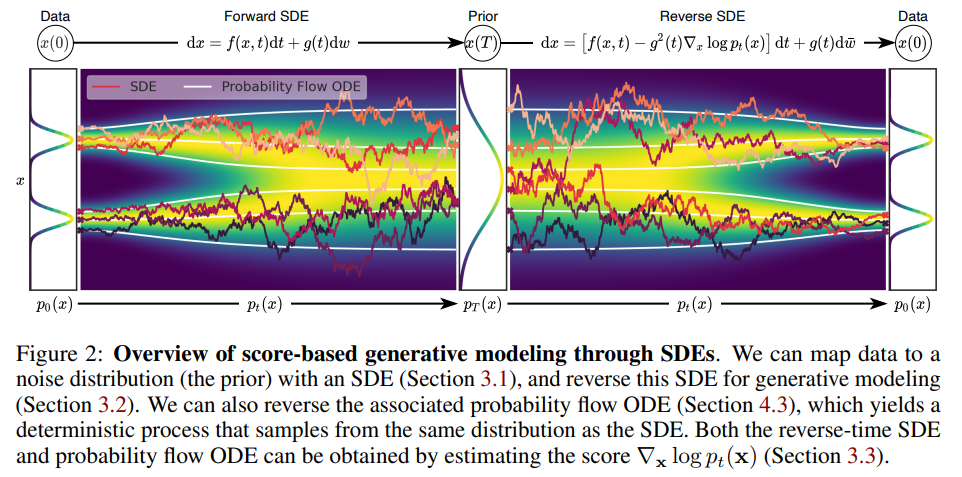
- time variable t에 대해서, T step에 대해 diffusion process를 구현하는 것을 목표로 한다. 즉, \(p_0\)은 data distribution이고, \(p_T\)는 prior distribution이다. Diffusion process는 다음과 같이 표현된다.
- w는 standard Wiener process(=Brownian motion), f는 drift function이라고 불리는 vector valued function이다. g는 diffusion coefficient라고 불리는 scalar function이다. SDE는 globally Lipschitz할 때 unique strong solution을 가진다. \(x(s)\)부터 \(x(t)\)의 transition kernel을 나타내기 위해 \(p_{st}(x(t)\vert{}x(s))\)를 사용한다.
3.2 Generating Samples by Reversing the SDE
- SDE로 diffusion process를 구현했는데, 역과정 또한 diffusion process로 생각할 수 있고, 그 과정은 reverse-time SDE로 나타낼 수 있다.
- \(\bar{w}\)는 T부터 0까지 역방향으로 작용하는 standard Wiener process이고 dt는 infinitesimal negative timestep이다. 모든 t에 대하여, \(\nabla_x \log p_t(x)\)를 알 때, reverse diffusion process를 구현해 \(p_0\)를 얻을 수 있다.
3.3 Estimating Scores For the SDE
- Score distribution은 score-based model을 학습함으로써 추정할 수 있다. \(\nabla_x \log{p_t}(x)\)를 추정하기 위해 time-dependent score-based model을 학습한다.
- lambda는 양의 실수 범위를 가지는 weighting function, t는 [0, T] 범위에서 uniformly sampled되었다. 충분한 양의 데이터와 model capacity가 있으면, score matching은 optimized되고, SMLD와 DDPM에서와 같이, \(\lambda(t) \propto 1/\mathbb{E} \left[ \Vert{} \nabla_{x(t)} \log p_{0t}(x(t)\mid x(0))\Vert{}_2^2 \right]\)를 선택할 수 있다. 이와 다른 score matching 방법을 선택할 수도 있다.
3.4 Examples: VE, VP SDEs and Beyond
- SMLD와 DDPM의 noise perturbation 과정은 모두 SDE의 형태로 표현될 수 있다.
- SMLD: \(x_i = x_{i-1} + \sqrt{\sigma_i^2 - \sigma_{i-1}^2} z_{i-1}, \quad i = 1, \dots, N\) \(dx = \sqrt{ \frac{d[\sigma^2(t)] \,}{ dt}}dw\), 왼쪽의 수식에서 drift coefficient가 0이기 때문에 평균은 보존되고 분산은 계속해서 증가한다.
- DDPM: \(x_i = \sqrt{( 1 - \beta_i)} x_{i-1} + \sqrt{\beta_i} z_{i-1}, \quad i = 1, \dots, N\) \(dx = -\frac{1}{2} \beta(t)x \, dt + \sqrt{ \beta(t)} \, dw\), 왼쪽의 수식에서 variance가 보존됨을 알 수 있다.
- SMLD은 Variance Exploding(VE) SDE이고, DDPM은 Variance Preserving(VP) SDE이다.
- VP SDE에서 영감을 받아 논문의 저자들은 아래와 같은 SDE를 제안했다.
- 위의 SDE에서의 variance는 항상 VP SDE의 variance로 bounded되기 때문에 위와 같은 SDE를 sub-VP SDE라고 부른다.
4. Solving the Reverse SDE
- Time dependent score-based model을 학습시킨 후, 우리는 reverse-time SDE를 구현한 후, 샘플을 만들기 위해 수치적으로 접근할 수 있다.
4.1 General-Purpose Numerical SDE Solvers
- SDE를 푸는데 다양한 general-purpose numerical method가 존재한다(Euler-Maruyama, stochastic Runge-Kutta). 이러한 방법들 중 아무거나 reverse-time SDE를 푸는데 적용해 샘플을 만들어 내는데 사용할 수 있다. 저자들은 본 논문에서 forward SDE와 같은 방식으로 reverse-time SDE를 discretetize한 reverse diffusion sampler을 제안한다.