Understanding Diffusion Models: A Unified Perspective

arxiv.org

Background: ELBO, VAE, and Hierarchical VAE

Evidence Lower Bound

\[p(x) = \int p(x,z)dz\]

• Latent Variable: 잠재 변수
• x라는 observed data, z라는 latent variable에 대해서 x의 확률 분포를 위의 그림과 같이 쓸 수 있다. 위의 표현은 Chain Rule of Probability를 사용해 다음과 같이 나타낼 수도 있다.

\[p(x) = \frac{p(x,z)}{p(z|x)}\]

• 우리가 x의 확률 분포를 구하고자 할 때 이를 직접 구하는 것에는 어려움이 있다. 왜냐하면 x의 확률 분포는 latent variable과 연관이 되어 있고(위의 식에서 x에 대한 z의 조건부 확률을 알아야 한다) latent variable은 우리가 쉽게 찾을 수 없다. 따라서 우리는 x의 확률 분포를 가장 잘 나타내는 식을 추정해야 한다. 이 방법으로 ELBO가 있는 것이다. x의 확률에 로그를 씌운 값은 다음과 같은 대소 관계를 가진다. Lower Bound를 가지는 셈인데 Lower Bound를 최대화 하기로 한다.

\[\begin{align*}\log p(\mathbf{x}) &= \log \int p(\mathbf{x}, \mathbf{z}) \, d\mathbf{z} \quad &\text{(Apply Equation 1)} \\&= \log \int \frac{p(\mathbf{x}, \mathbf{z}) q_\phi(\mathbf{z} \mid \mathbf{x})}{q_\phi(\mathbf{z} \mid \mathbf{x})} \, d\mathbf{z} \quad &\text{(Multiply by 1 = } \frac{q_\phi(\mathbf{z} \mid \mathbf{x})}{q_\phi(\mathbf{z} \mid \mathbf{x})} \text{)} \\&= \log \mathbb{E}_{q_\phi(\mathbf{z} \mid \mathbf{x})} \left[ \frac{p(\mathbf{x}, \mathbf{z})}{q_\phi(\mathbf{z} \mid \mathbf{x})} \right] \quad &\text{(Definition of Expectation)} \\&\geq \mathbb{E}_{q_\phi(\mathbf{z} \mid \mathbf{x})} \left[ \log \frac{p(\mathbf{x}, \mathbf{z})}{q_\phi(\mathbf{z} \mid \mathbf{x})} \right] \quad &\text{(Apply Jensen's Inequality)}\end{align*}\]

• 위의 식에서 q(x에 대한 z의 조건부 확률의 추정치)는 우리가 실제로 구하기 어려운 값이다. 그래서 이 값을 매개화 해서 구할 것이고 ELBO를 최대화할 수 있는 파라미터를 찾을 것이다. 위의 과정을 통해서 Lower Bound가 설정되었다. Jensen’s Inequality는 아래와 같은 관계를 나타내는 수식이다.

\[f(E[X]) ≥ E[f(X)]\]

• 하지만 위의 관계식 만으로는 ELBO에 대한 정보를 충분히 얻을 수 없다. 왜 이것이 실제로 Lower Bound가 되는지, 왜 이 값을 maximize 해야 하는지를 알 수 없다. 그래서 위의 식을 다음과 같이 나타내면 그 답을 얻을 수 있다.

\[\begin{align*}\log p(\mathbf{x}) &= \log \int \frac{p(\mathbf{x}, \mathbf{z})}{q_\phi(\mathbf{z} \mid \mathbf{x})} q_\phi(\mathbf{z} \mid \mathbf{x}) \, d\mathbf{z} \quad &\text{(Multiply by 1 = } \int q_\phi(\mathbf{z} \mid \mathbf{x}) \, d\mathbf{z}) \\&= \int q_\phi(\mathbf{z} \mid \mathbf{x}) (\log p(\mathbf{x})) \, d\mathbf{z} \quad &\text{(Bring evidence into integral)} \\&= \mathbb{E}_{q_\phi(\mathbf{z} \mid \mathbf{x})} [\log p(\mathbf{x})] \quad &\text{(Definition of Expectation)} \\&= \mathbb{E}_{q_\phi(\mathbf{z} \mid \mathbf{x})} \left[ \log \frac{p(\mathbf{x}, \mathbf{z})}{p(\mathbf{z})} \right] \quad &\text{(Apply Equation 2)} \\&= \mathbb{E}_{q_\phi(\mathbf{z} \mid \mathbf{x})} \left[ \log \frac{p(\mathbf{x}, \mathbf{z}) q_\phi(\mathbf{z} \mid \mathbf{x})}{p(\mathbf{z}) q_\phi(\mathbf{z} \mid \mathbf{x})} \right] \quad &\text{(Multiply by 1 = } \frac{q_\phi(\mathbf{z} \mid \mathbf{x})}{q_\phi(\mathbf{z} \mid \mathbf{x})}) \\&= \mathbb{E}_{q_\phi(\mathbf{z} \mid \mathbf{x})} \left[ \log \frac{p(\mathbf{x}, \mathbf{z})}{q_\phi(\mathbf{z} \mid \mathbf{x})} \right] + \mathbb{E}_{q_\phi(\mathbf{z} \mid \mathbf{x})} \left[ \log \frac{q_\phi(\mathbf{z} \mid \mathbf{x})}{p(\mathbf{z} \mid \mathbf{x})} \right] \quad &\text{(Split the Expectation)} \\&= \mathbb{E}_{q_\phi(\mathbf{z} \mid \mathbf{x})} \left[ \log \frac{p(\mathbf{x}, \mathbf{z})}{q_\phi(\mathbf{z} \mid \mathbf{x})} \right] + D_{\text{KL}}(q_\phi(\mathbf{z} \mid \mathbf{x}) \parallel p(\mathbf{z} \mid \mathbf{x})) \quad &\text{(Definition of KL Divergence)} \\&\geq \mathbb{E}_{q_\phi(\mathbf{z} \mid \mathbf{x})} \left[ \log \frac{p(\mathbf{x}, \mathbf{z})}{q_\phi(\mathbf{z} \mid \mathbf{x})} \right] \quad &\text{(KL Divergence always } \geq 0)\end{align*}\]

• 여기서 KL Divergence는 두 확률 분포가 얼마나 차이를 보이는지에 대한 지표이다.

\[D_{\text{KL}}(P || Q) = \sum_x P(x) \log \frac{P(x)}{Q(x)}\]

• 위의 식에서 x에 대한 확률은 ELBO 항과 KL Divergence 항으로 나타난다. 이때 KL Divergence가 항상 0보다 크기 때문에 Lower Bound가 설정이 된다. 위의 식에서 KL Divergence가 0이 된다는 의미는 두 확률 분포가 같음을 의미하며 variational posterior q가 실제 z의 사후 분포인 p와 동일해지는 것과 같다. 실제 사후 분포를 구하기 어려우니 이를 variational posterior으로 나타내고자 하는 것이고 variational posterior가 실제 사후 분포와 유사할수록 KL Divergence는 작아진다. ELBO를 최대화 하는 것은 곧 latent variable인 z의 분포를 정확하게 알 수 있음과 같다.

Variational Autoencoders

\[\begin{align}\mathbb{E}_{q_\phi(z|x)} \left[ \log \frac{p(x, z)}{q_\phi(z|x)} \right] &= \mathbb{E}_{q_\phi(z|x)} \left[ \log \frac{p_\theta(x|z) p(z)}{q_\phi(z|x)} \right] \quad \text{(Chain Rule of Probability)} \\&= \mathbb{E}_{q_\phi(z|x)} \left[ \log p_\theta(x|z) \right] + \mathbb{E}_{q_\phi(z|x)} \left[ \log \frac{p(z)}{q_\phi(z|x)} \right] \quad \text{(Split the Expectation)} \\&= \underbrace{\mathbb{E}_{q_\phi(z|x)} \left[ \log p_\theta(x|z) \right]}_{\text{reconstruction term}} - \underbrace{D_{\text{KL}}(q_\phi(z|x) \| p(z))}_{\text{prior matching term}} \quad \text{(Definition of KL Divergence)}.\end{align}\]

• 이전까지 우리는 가장 분포를 잘 설명하는 variational posterior을 구하기 위해 왜 ELBO를 최대화 해야 하는지를 알아보았다. 그러면 ELBO를 더 잘 해석하기 위해 위와 같이 reconstruction term과 prior matching term으로 분해했다. KL Divergence 값은 항상 0보다 크기 때문에 ELBO를 최대화 하려면 reconstruction term은 최대화, prior matching term은 최소화를 해야 한다. 각각의 term은 무슨 의미를 가지고 있을까?
• 각각의 term의 의미를 알아보기 전에 q, p가 위의 식에서 어떤 기능을 하는지 알아야 한다. \(q_\phi(z\vert{}x)\)는 encoder로 input인 x를 가능한 latent에 대하여 transform 한다. \(p_\theta(x\vert{}z)\)는 decoder로 latent z로부터 x를 복원(재구성)한다.
• reconstruction term은 말 그대로 decoder가 latent로부터 얼마나 잘 재현되는지를 측정한다. prior matching term은 학습된 z에 대한 variational distribution이 얼마나 이전의 정보와 일치하는지를 측정한다.
• ELBO는 파라미터 φ 와 θ를 통해 매개화된다. encoder은 주로 multivariate Gaussian을 따르도록 선택이 되며, prior은 standard multivariate Gaussian을 따르도록 선택된다.

\[q_\phi(z|x) = \mathcal{N}(z; \mu_\phi(x), \sigma_\phi^2(x)\mathbf{I}) \\ p(z) = \mathcal{N}(z; 0, \mathbf{I})\]

• ELBO의 KL Divergence term은 몬테카를로 방법을 통해 추정할 수 있다.

\[\int f(x) p(x) \, dx \approx \frac{1}{N} \sum_{i=1}^{N} f(x_i) \ \ Monte\ Carlo \ estimation\] \[\arg \max_{\phi, \theta} \mathbb{E}_{q_\phi(z|x)} \left[ \log p_\theta(x|z) \right] - D_{\text{KL}}(q_\phi(z|x) \| p(z)) \approx \arg \max_{\phi, \theta} \sum_{l=1}^{L} \log p_\theta(x|z^{(l)}) - D_{\text{KL}}(q_\phi(z|x) \| p(z))\]

• 몬테카를로 방법으로 ELBO를 위와 같이 표현할 수 있다. 하지만 각각의 latent z는 확률적으로 선택이 되고 이는 미분 가능하지 않다는 문제가 발생한다. 하지만 이를 재매개화(reparameterization) 방법을 통해 해결할 수 있다. 임의의 Gaussian Distribution은 Normal Distribution이 평균 만큼 shift된 것으로 생각할 수 있고 아래와 같이 쓸 수 있다.

\[z = \mu_\phi(x) + \sigma_\phi(x) \odot \epsilon \quad \text{with} \quad \epsilon \sim \mathcal{N}(\epsilon; 0, \mathbf{I})\]

Hierarchical Variational Autoencoders

• HVAE는 VAE의 일반화된 형태로 latent variable 간에 계층(hierarchical) 관계가 있음을 나타낸다. 여기서는 latent variable이 더 복잡하고, 추상적인 higher level latent로부터 생성되었다고 본다.

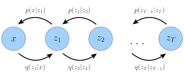
• 위의 과정은 마르코프 성질을 가지기 때문에 오직 이전 state의 영향만을 받으며 latent가 생성된다. 정방향과 역방향 과정 q, p에 대하여 다음과 같은 성질이 있다.

\[p(x, z_{1:T}) = p(z_T) p_\theta(x | z_1) \prod_{t=2}^{T} p_\theta(z_{t-1} | z_t)\] \[q_\phi(z_{1:T} | x) = q_\phi(z_1 | x) \prod_{t=2}^{T} q_\phi(z_t | z_{t-1})\]

• 이를 적용해 ELBO를 다시 표현할 수 있다.

\[\begin{aligned} &\log p(x) = \log \int p(x, z_{1:T}) \, dz_{1:T} \\ &= \log \int \frac{p(x, z_{1:T}) q_\phi(z_{1:T} | x)}{q_\phi(z_{1:T} | x)} \, dz_{1:T} \quad \text{(Multiply by 1 = } \frac{q_\phi(z_{1:T} | x)}{q_\phi(z_{1:T} | x)}\text{)} \\ &= \log \mathbb{E}_{q_\phi(z_{1:T} | x)} \left[ \frac{p(x, z_{1:T})}{q_\phi(z_{1:T} | x)} \right] \quad \text{(Definition of Expectation)} \\ &\geq \mathbb{E}_{q_\phi(z_{1:T} | x)} \left[ \log \frac{p(x, z_{1:T})}{q_\phi(z_{1:T} | x)} \right] \quad \text{(Apply Jensen's Inequality)} \end{aligned}\] \[\mathbb{E}_{q_\phi(z_{1:T} | x)} \left[ \log \frac{p(x, z_{1:T})}{q_\phi(z_{1:T} | x)} \right] = \mathbb{E}_{q_\phi(z_{1:T} | x)} \left[ \log \frac{p(z_T) p_\theta(x | z_1) \prod_{t=2}^{T} p_\theta(z_{t-1} | z_t)} {{q_\phi(z_1 | x)}{\prod_{t=2}^{T} q_\phi(z_t | z_{t-1})}} \right]\]

• 이제 지금까지 정리한 내용을 이용해 Variational Diffusion Model을 분석할 수 있다.

Variational Diffusion Models

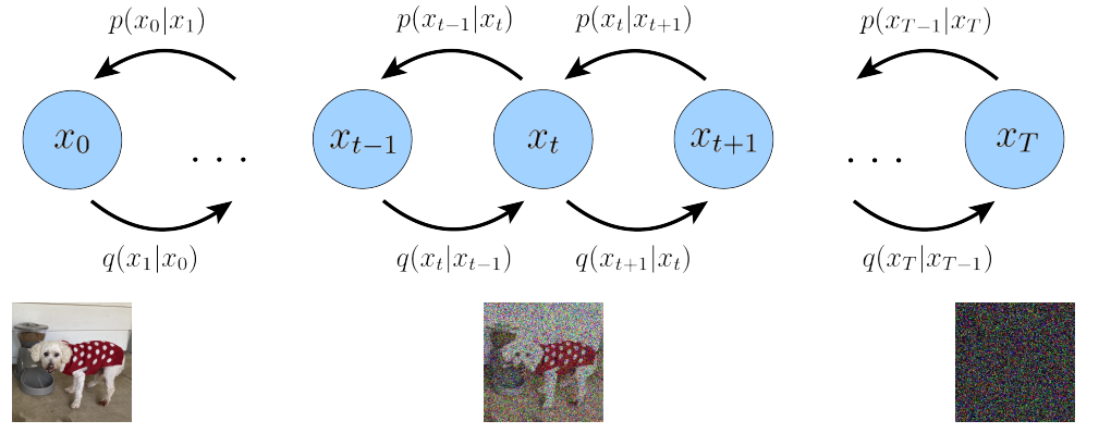
• 디퓨전 모델은 노이즈를 추가하는 과정이 분자의 확산과 유사하다고 해서 디퓨전이라는 이름이 붙었다. 어떤 이미지가 있다고 했을 때, 이미지의 각 픽셀에 노이즈를 추가한다. 매 state마다 노이즈를 추가하며 원래 이미지의 특성을 점점 줄여나간다. 우리의 목표는 노이즈가 추가된 이미지에서 원래 이미지를 복원하는 것이다. 노이즈 추가의 과정은 일정 규칙에 따라 이루어진다. 하지만 노이즈가 추가된 상태에서 노이즈가 추가되기 전 상태인 이전 상태로 돌아가는 것은 어렵다. 그러면 노이즈를 제거하며 이전 상태를 복원하는 과정을 어떻게 할 수 있을까?
• 디퓨전 모델은 MHVAE가 3가지 restriction을 가지고 있는 상태라고 생각할 수 있다.
  • The latent dimension is exactly equal to the data dimension
  • The structure of the latent encoder at each timestep is not learned; it is pre-defined as a linear Gaussian model. In other words, it is a Gaussian distribution centered around the output of the previous timestep
  • The Gaussian parameters of the latent encoders vary over time in such a way that the distribution of the latent at final timestep T is a standard Gaussian
• 2번 조건에서 encoder는 pre-defined되어 있으며 이전 state 근방에 분포한 Gaussian 분포로 다음 state가 정의된다고 한다. 아래 식을 보면 다음 state의 분포가 이전 state로 정의되는 것을 볼수 있다. 여기서 alpha가 커지면 이전 state와 유사한 분포를 가지고, alpha가 작아지면 standard Gaussian에 가까워지는 것을 볼 수 있다. encoder은 노이즈를 추가하는 과정이다. alpha 값에 따라서 노이즈를 얼마나 추가하며, 이전 state 상태를 얼마나 보존할지를 선택할 수 있는 것이다.

\[q(x_t | x_{t-1}) = \mathcal{N} \left( x_t; \sqrt{\alpha_t} x_{t-1}, (1 - \alpha_t) \mathbf{I} \right)\]

• 3번 조건에서 마지막 state에서 x의 분포는 standard Gaussian을 따른다고 한다. p는 decoder로 노이즈를 제거하는 과정이라고 생각할 수 있다. 이 과정 역시 마르코프 성질을 따르기에 아래와 같은 형태로 쓸 수 있다.

\[p(x_{0:T}) = p(x_T) \prod_{t=1}^{T} p_\theta(x_{t-1} | x_t)\]

• 정리하자면 encoder은 노이즈를 추가하는 과정, decoder은 standard Gaussian을 따르는 final state에서 노이즈를 점점 제거하는 과정이라고 볼 수 있다. 이때 encoder은 우리가 정의를 해서 사용한다. 각각의 timestep에서 이전 state의 특성을 얼마나 반영해 다음 state를 정의하는지를 앞서 다룬 바 있다. 하지만 decoder의 경우, 우리가 아는 것이 없다. 당연히도 이미지에 노이즈를 추가하는 것은 쉽지만 노이즈가 추가된 이미지에서 원래 이미지를 복원하는 것은 어려울 것이다(실제 확산 현상과 연관지어 생각해 본다면 물병에 떨어트린 물감을 다시 물과 물감으로 분리하는 것은 어렵다는 것과 유사하다고 볼 수 있다). 결국에 standard Gaussian상태에서 순차적인 denoising을 통해 initial state로 복원해 줄 수 있는 p를 추정하는 것이 목표이다. 이 과정에서 ELBO가 다시 등장한다.

\[\begin{aligned}\log p(x) &= \log Z \int p(x_{0:T}) \, dx_{1:T} \\&= \log Z \int \frac{p(x_{0:T}) q(x_{1:T} | x_0)}{q(x_{1:T} | x_0)} \, dx_{1:T} \\&= \log \mathbb{E}_{q(x_{1:T} | x_0)} \left[ \frac{p(x_{0:T})}{q(x_{1:T} | x_0)} \right] \\&\geq \mathbb{E}_{q(x_{1:T} | x_0)} \left[ \log \frac{p(x_{0:T})}{q(x_{1:T} | x_0)} \right] \\&= \mathbb{E}_{q(x_{1:T} | x_0)} \left[ \log p(x_T) \prod_{t=1}^{T} p_\theta(x_{t-1} | x_t) \prod_{t=1}^{T} q(x_t | x_{t-1}) \right] \\&= \mathbb{E}_{q(x_{1:T} | x_0)} \left[ \log p(x_T) p_\theta(x_0 | x_1) \prod_{t=2}^{T} p_\theta(x_{t-1} | x_t) q(x_T | x_{T-1}) \prod_{t=1}^{T-1} q(x_t | x_{t-1}) \right] \\&= \mathbb{E}_{q(x_{1:T} | x_0)} \left[ \log p(x_T) p_\theta(x_0 | x_1) \prod_{t=1}^{T-1} p_\theta(x_t | x_{t+1}) q(x_T | x_{T-1}) \prod_{t=1}^{T-1} q(x_t | x_{t-1}) \right] \\&= \mathbb{E}_{q(x_{1:T} | x_0)} \left[ \log p(x_T) p_\theta(x_0 | x_1) \frac{q(x_T | x_{T-1})}{q(x_T | x_{T-1})} \prod_{t=1}^{T-1} \frac{p_\theta(x_t | x_{t+1})}{q(x_t | x_{t-1})} \right] \\&= \mathbb{E}_{q(x_{1:T} | x_0)} \left[ \log p_\theta(x_0 | x_1) \right] + \mathbb{E}_{q(x_{1:T} | x_0)} \left[ \log \frac{p(x_T)}{q(x_T | x_{T-1})} \right] \\&\quad + \sum_{t=1}^{T-1} \mathbb{E}_{q(x_{1:T} | x_0)} \left[ \log \frac{p_\theta(x_t | x_{t+1})}{q(x_t | x_{t-1})} \right] \\&= \mathbb{E}_{q(x_1 | x_0)} \left[ \log p_\theta(x_0 | x_1) \right] + \mathbb{E}_{q(x_T | x_{T-1})} \left[ \log \frac{p(x_T)}{q(x_T | x_{T-1})} \right] \\&\quad + \sum_{t=1}^{T-1} \mathbb{E}_{q(x_{t-1}, x_t, x_{t+1} | x_0)} \left[ \log \frac{p_\theta(x_t | x_{t+1})}{q(x_t | x_{t-1})} \right] \\&= \mathbb{E}_{q(x_1 | x_0)} \left[ \log p_\theta(x_0 | x_1) \right] \quad \text{(reconstruction term)} \\&\quad - \mathbb{E}_{q(x_{T-1} | x_0)} \left[ D_{\text{KL}}(q(x_T | x_{T-1}) \| p(x_T)) \right] \quad \text{(prior matching term)} \\&\quad - \sum_{t=1}^{T-1} \mathbb{E}_{q(x_{t-1}, x_t, x_{t+1} | x_0)} \left[ D_{\text{KL}}(q(x_t | x_{t-1}) \| p_\theta(x_t | x_{t+1})) \right] \quad \text{(consistency term)}\end{aligned}\]

• 최종 결과에서 3개의 term이 나온다. 각각의 term이 무슨 의미를 가지는지, 또 어떻게 되어야 하는지를 알아보자
  • reconstruction term: state1에 대한 state0의 로그 확률을 나타낸다. 이 term은 vanilla VAE에도 등장을 하고 유사하게 학습될 수 있다.
  • prior matching term: 이 term은 final state가 이전 state의 Gaussian을 따를 때 minimized된다. 우리가 충분히 노이즈를 추가했을 때 final state는 standard Gaussian을 따른다고 했고 T가 충분히 크다면 q, p가 모두 standard Gaussian을 따르기 때문에 이 term은 0이 된다.

    • 아래의 식에서 final state에서 alpha값은 0으로 가기 때문에 standard Gaussian으로 가게 된다.

      \[q(x_t | x_{t-1}) = \mathcal{N} \left( x_t; \sqrt{\alpha_t} x_{t-1}, (1 - \alpha_t) \mathbf{I} \right)\]
  • consistency term: 이 term은 각 항에서 p가 q를 따를 때 최소화된다. 우리는 위의 식을 알고 있기에 p가 위의 Gaussian을 따르도록 train 한다면 이 term이 최소화된다.
• 우리는 consistency term을 0으로 만들도록 decoder을 학습시켜야 한다. 이는 Monte Carlo 방법으로 수행될 수 있으나 suboptimal할 수 있다. 그 이유는 consistency term에서 \(x_{t-1}, x_{t+1}\)이라는 두 random variable에 대한 expectation을 계산해야 하기 때문에 하나의 random variable을 가지고 expectation을 계산하는 것보다 variation이 커지게 된다. 그러면 ELBO를 하나의 random variable만으로 표현하는 방법을 찾을 수 있다. 그 과정은 아래의 equation에서 시작한다.

\[q(x_t | x_{t-1}) = q(x_t | x_{t-1}, x_0)\]

• 위 equation을 Bayes rule에 따라 다음과 같이 바꿀 수 있다.

\[q(x_t | x_{t-1}, x_0) = \frac {q(x_{t-1} | x_t, x_0) q(x_t | x_0)} {q(x_{t-1} | x_0)}\]

• 이를 적용해 ELBO를 다시 쓸 수 있다.

\[\begin{aligned}\log p(x) &\geq \mathbb{E}_{q(x_{1:T} | x_0)} \left[ \log \frac{p(x_{0:T})}{q(x_{1:T} | x_0)} \right] \\&= \mathbb{E}_{q(x_{1:T} | x_0)} \left[ \log p(x_T) \prod_{t=1}^{T} p_\theta(x_{t-1} | x_t) \prod_{t=1}^{T} q(x_t | x_{t-1}) \right] \\&= \mathbb{E}_{q(x_{1:T} | x_0)} \left[ \log p(x_T) p_\theta(x_0 | x_1) \prod_{t=2}^{T} p_\theta(x_{t-1} | x_t) q(x_1 | x_0) \prod_{t=2}^{T} q(x_t | x_{t-1}, x_0) \right] \\&= \mathbb{E}_{q(x_{1:T} | x_0)} \left[ \log p_\theta(x_T) p_\theta(x_0 | x_1) q(x_1 | x_0) + \log \prod_{t=2}^{T} p_\theta(x_{t-1} | x_t) q(x_{t-1} | x_t, x_0) q(x_t | x_0) \right] \\&= \mathbb{E}_{q(x_{1:T} | x_0)} \left[ \log p(x_T) p_\theta(x_0 | x_1) q(x_1 | x_0) + \sum_{t=2}^{T} \log p_\theta(x_{t-1} | x_t) q(x_{t-1} | x_t, x_0) \frac{q(x_t | x_0)}{q(x_{t-1} | x_0)} \right] \\&= \mathbb{E}_{q(x_{1:T} | x_0)} \left[ \log p(x_T) p_\theta(x_0 | x_1) q(x_1 | x_0) + \sum_{t=2}^{T} \log p_\theta(x_{t-1} | x_t) \frac{q(x_{t-1} | x_t, x_0)}{q(x_{t-1} | x_0)} \right] \\&= \mathbb{E}_{q(x_1 | x_0)} \left[ \log p_\theta(x_0 | x_1) \right] + \mathbb{E}_{q(x_T | x_0)} \left[ \log \frac{p(x_T)}{q(x_T | x_0)} \right] \\&\quad + \sum_{t=2}^{T} \mathbb{E}_{q(x_{t-1}, x_t | x_0)} \left[ \log \frac{p_\theta(x_{t-1} | x_t)}{q(x_{t-1} | x_t, x_0)} \right] \\&= \mathbb{E}_{q(x_1 | x_0)} \left[ \log p_\theta(x_0 | x_1) \right] + \mathbb{E}_{q(x_T | x_0)} \left[ \log \frac{p(x_T)}{q(x_T | x_0)} \right] \\&\quad + \sum_{t=2}^{T} \mathbb{E}_{q(x_t, x_{t-1} | x_0)} \left[ \log \frac{p_\theta(x_{t-1} | x_t)}{q(x_{t-1} | x_t, x_0)} \right] \\&= \mathbb{E}_{q(x_1 | x_0)} \left[ \log p_\theta(x_0 | x_1) \right] \quad \text{(reconstruction term)} \\&\quad - D_{\text{KL}}\left( q(x_T | x_0) \| p(x_T) \right) \quad \text{(prior matching term)} \\&\quad - \sum_{t=2}^{T} \mathbb{E}_{q(x_t | x_0)} \left[ D_{\text{KL}}\left( q(x_{t-1} | x_t, x_0) \| p_\theta(x_{t-1} | x_t) \right) \right] \quad \text{(denoising matching term)}\end{aligned}\]

• 위와 같은 표현 방식은 하나의 random variable만을 사용해 variance가 작다. 역시나 3개의 term으로 구성되어 있다.
  • reconstruction term: 동일
  • prior matching term: 이 term은 이전 방식과 약간 표현이 다르기는 하지만 trainable parameter가 없으며 q, p 모두 standard Gaussian을 따르기 때문에 0이 된다.

  • denoising matching term: q에 대한 표현에 변화가 생겼다. 우리는 \(q(x_{t}\vert{}x_{t-1}, x_0)\)은 잘 알고 있다. \(q(x_{t-1}\vert{}x_{t}, x_0)\)은 해석이 필요하다. 직관적으로 봤을 때 노이즈를 추가하는 과정의 반대 이므로 노이즈를 제거하는 과정이라고 생각할 수 있다.

    \[q(x_{t-1} | x_t, x_0) = \frac { q(x_t | x_{t-1}, x_0)q(x_{t-1} | x_0)} {q(x_{t} | x_0)}\]
• Bayes rule을 통해 위와 같은 관계를 얻을 수 있다. \(q(x_{t}\vert{}x_{t-1}, x_0)\)은 Gaussian Distribution을 따른다는 것을 알고 있고 \(q(x_{t-1}\vert{}x_0)\), \(q(x_{t}\vert{}x_0)\)을 알아야 한다. 이때 \(x_{t}\)가 \(q(x_{t}\vert{}x_{t-1})\)와 같은 분포를 따름을 알고 다음과 같이 쓸 수 있다. encoder에서 mean과 variance를 이전 state로 정의했고 이를 multivariate Gaussian 형태로 쓴 것이다.

\[x_t = \sqrt{\alpha_t} x_{t-1} + \sqrt{1 - \alpha_t} \epsilon, \quad \epsilon \sim \mathcal{N}(\epsilon; 0, I)\]

• 위의 수식을 연쇄적으로 쓴다면 \(x_0\)로 나타낼 수 있게 된다.

\[\begin{aligned} &x_t = \sqrt{\alpha_t} x_{t-1} + \sqrt{1 - \alpha_t} \epsilon_{t-1} \\ &= \sqrt{\alpha_t \alpha_{t-1}} x_{t-2} + \sqrt{\alpha_t - \alpha_t \alpha_{t-1}} \epsilon_{t-2} + \sqrt{1 - \alpha_t} \epsilon_{t-1} \\ &= \sqrt{\alpha_t \alpha_{t-1}} x_{t-2} + \sqrt{1 - \alpha_t \alpha_{t-1}} \epsilon_{t-2} \\ &= \dots \\ &= \sqrt{\bar{\alpha}_t} x_0 + \sqrt{1 - \bar{\alpha}_t} \epsilon_0 \\ &\sim \mathcal{N}(x_t; \sqrt{\bar{\alpha}_t} x_0, (1 - \bar{\alpha}_t) I)\\ &\bar{\alpha} = \prod_{i=1}^{T} \alpha_i \end{aligned}\]

• 이제 위의 결과를 이용해 \(q(x_{t-1} \vert{} x_t, x_0)\)의 분포를 얻을 수 있다. \(q(x_{t} \vert{} x_{t-1}, x_0)\), \(q(x_{t-1} \vert{} x_0)\), \(q(x_{t} \vert{} x_0)\) 모두 Gaussian Distribution을 따르고 다음의 관계를 따른다.

\[\begin{align*}q(x_{t-1} | x_t, x_0) &= \frac{q(x_t | x_{t-1}, x_0) q(x_{t-1} | x_0)}{q(x_t | x_0)} &\propto \mathcal{N} \left( x_{t-1}; \underbrace{\frac{\sqrt{\alpha_t} (1 - \bar{\alpha}_{t-1}) x_t + \sqrt{\bar{\alpha}_{t-1}} (1 - \alpha_t) x_0}{1 - \bar{\alpha}_t}}_{\mu_q(x_t, x_0)}, \underbrace{\frac{(1 - \alpha_t)(1 - \bar{\alpha}_{t-1})}{1 - \bar{\alpha}_t}I}_{\Sigma_q(t)} \right)\end{align*}\]

• \(q(x_{t-1} \vert{} x_t, x_0)\)가 Gaussian Distribution을 따르는 것을 알았기 때문에 decoder 또한 Gaussian Distribution을 따르게 추정하는 것이 적합하다고 판단할 수 있다. 하지만 decoder \(p_{\theta}(x_{t-1} \vert{} x_t)\)는 \(x_0\)에 대해 표현되지 않는다. 일단은 두 분포간의 KL Divergence를 최소화해야 하고 두 분포 모두 Gaussian임은 알고 있다. Gaussian Distribution간의 KL Divergence는 아래와 같이 계산할 수 있다. 이를 적용해 KL Divergence를 최소화하는 decoder를 찾을 수 있다.

\[\begin{align*}D_{KL}(\mathcal{N}(x; \mu_x, \Sigma_x) \, \| \, \mathcal{N}(y; \mu_y, \Sigma_y)) = \frac{1}{2} \left[ \log \frac{|\Sigma_y|}{|\Sigma_x|} - d + \text{tr}(\Sigma_y^{-1} \Sigma_x) + (\mu_y - \mu_x)^T \Sigma_y^{-1} (\mu_y - \mu_x) \right]\end{align*}\] \[\begin{align*}\arg\min_{\theta} D_{KL}(q(x_{t-1} \mid x_t, x_0) \, \| \, p_\theta(x_{t-1} \mid x_t)) &= \arg\min_{\theta} D_{KL}(\mathcal{N}(x_{t-1}; \mu_q, \Sigma_q(t)) \, \| \, \mathcal{N}(x_{t-1}; \mu_\theta, \Sigma_q(t))) \\&= \arg\min_{\theta} \frac{1}{2} \left[ \log \frac{|\Sigma_q(t)|}{|\Sigma_q(t)|} - d + \text{tr}(\Sigma_q(t)^{-1} \Sigma_q(t)) + (\mu_\theta - \mu_q)^T \Sigma_q(t)^{-1} (\mu_\theta - \mu_q) \right] \\&= \arg\min_{\theta} \frac{1}{2} \left[ \log 1 - d + d + (\mu_\theta - \mu_q)^T \Sigma_q(t)^{-1} (\mu_\theta - \mu_q) \right] \\&= \arg\min_{\theta} \frac{1}{2} (\mu_\theta - \mu_q)^T \Sigma_q(t)^{-1} (\mu_\theta - \mu_q) \\&= \arg\min_{\theta} \frac{1}{2} \left[ (\mu_\theta - \mu_q)^T (\sigma_q^2(t) I)^{-1} (\mu_\theta - \mu_q) \right] \\&= \arg\min_{\theta} \frac{1}{2 \sigma_q^2(t)} \| \mu_\theta - \mu_q \|_2^2\end{align*}\]

• KL Divergence를 두 분포의 평균으로 나타내었다. encoder 분포에서의 평균은 위에서 구했었다. decoder는 앞서 \(x_0\)에 conditional하지 않다고 했었고 따라서 이 값을 estimator을 이용해 표현해야 한다. \(\hat{x}_\theta(x_t, t)\)은 노이즈가 추가된 상태인 \(x_t\)의 초기 상태 \(x_0\)에 대한 값을 \(x_t\)로 매개화한 값이다.

\[\begin{aligned} &\mu_q(x_t, x_0) = \frac{\sqrt{\alpha_t (1 - \bar{\alpha}_{t-1})} x_t + \sqrt{\bar{\alpha}_{t-1} (1 - \alpha_t)} x_0}{1 - \bar{\alpha}_t}\\ &\mu_\theta(x_t, t) = \frac{\sqrt{\alpha_t (1 - \bar{\alpha}_{t-1})} x_t + \sqrt{\bar{\alpha}_{t-1} (1 - \alpha_t)} \hat{x}_\theta(x_t, t)}{1 - \bar{\alpha}_t} \end{aligned}\]

• 위의 term을 다시 대입하면 식을 다음과 같이 나타낼 수 있다.

\[\arg\min_\theta \, \frac{1}{2 \sigma_q^2(t)} \frac{\bar{\alpha}_{t-1}(1 - \alpha_t)^2}{(1 - \bar{\alpha}_t)^2}\left\| \hat{x}_\theta(x_t, t) - x_0 \right\|_2^2\]

• 결국 VDM이 초기 state를 찾아내는 문제가 되었다.

Learning Diffusion Noise Parameters

• 디퓨전 모델이 결국 초기 state를 찾아내는 문제가 됨을 보였다. 해당 식은 노이즈 파라미터가 포함된 꼴로 나타난다. 그렇다면 이제 노이즈 파라미터를 찾는 방법을 알아보자. \(\bar{\alpha_t} = \prod_{i=1}^{T} \alpha_i\)를 각 항에서 계산해야 한다. 하지만 매 timestep에서 이 값을 계산하는 것은 비효율적이다. SNR(Signal-to-Noise-Rate)을 다음과 같이 정의할 때 위의 식은 SNR로 표현될 수 있다.

\[SNR(t) = \frac{\bar\alpha_{t-1}}{1 - \bar\alpha_{t-1}} = \frac{\mu^2}{ \sigma^2}\] \[\begin{aligned} &\frac{1}{2} \left[ \frac{\alpha_{t-1}}{1 - \alpha_{t-1}} - \frac{\alpha_t}{1 - \alpha_t} \right] \left\| \hat{x}_\theta(x_t, t) - x_0 \right\|^2 \\ &= \frac{1}{2} \sigma^2_q(t) \alpha_{t-1} (1 - \alpha_t)^2 (1 - \alpha_{t})^2 \left\| \hat{x}_\theta(x_t, t) - x_0 \right\|_2^2 \\ &= \frac{1}{2} (\text{SNR}(t-1) - \text{SNR}(t)) \left\| \hat{x}_\theta(x_t, t) - x_0 \right\|_2^2 \end{aligned}\]

• SNR은 자세히 보면 encoder의 각 state에 대한 평균과 분산으로 이루어진 식임을 알 수 있다. SNR은 기존 시그널과 노이즈 양의 비율로 SNR이 크면 시그널이 많고, 작으면 노이즈가 많은 상태이다. 디퓨전 모델에서는 SNR이 단조 감소하도록 해 마지막 state T에서 standard Gaussian을 따르도록 노이즈를 점진적으로 추가해야 한다. 그러면 SNR을 아래와 같이 쓸 수 있고 SNR을 구성하는 alpha도 다시 표현할 수 있다.

\[\begin{aligned} &\frac{\overline{\alpha}_t}{1 - \overline{\alpha}_t} = \exp(-\omega \eta(t))\\ &\overline{\alpha}_t = \text{sigmoid}(-\omega \eta(t)) = \frac{1}{1 + \exp(\omega \eta(t))}\\ &1 - \overline{\alpha}_t = \text{sigmoid}(\omega \eta(t))=\frac{1}{1 + \exp(-\omega \eta(t))} \end{aligned}\]

• \(\omega \eta(t)\)는 단조 증가하는 neural network이고 이 함수도 최적화 되어야 한다.

Three Equivalent Interpretations

• 앞서 보았듯이 VDM은 초기 state를 임의의 state t로부터 예측하는 neural network를 구축하는 것으로 학습될 수 있다. 이전에 구한 t state에서의 분포를 변형해 아래와 같이 쓸 수 있다.

\[x_0 =\frac{x_t − \sqrt{1 − \bar\alpha_t}\epsilon_0}{\sqrt{\bar\alpha_t}}\] \[\mu_q(x_t, x_0)= \frac{1}{\sqrt{\alpha_t}} x_t - \frac{(1 - \alpha_t)}{ \sqrt{1 - \overline{\alpha}_t}\sqrt{\alpha_t}} \epsilon_0\] \[\mu_\theta(x_t, t)= \frac{1}{\sqrt{\alpha_t}} x_t - \frac{(1 - \alpha_t)}{ \sqrt{1 - \overline{\alpha}_t}\sqrt{\alpha_t}}\hat\epsilon(x_t, t)\]

• initial state는 우리가 알 수 없기 때문에 state t로 이를 estimate 해서 표현해야 한다. 지금까지 계속해서 해온 작업은 KL Divergence를 최소화 하기 위해 식을 계속해서 변형한 것이었다. 지금까지의 결과로 KL Divergence를 최소화하는 문제를 최종적으로 다음과 같이 나타낼 수 있다.

\[\arg \min_\theta \, D_{\text{KL}} \left( q(x_{t-1} \mid x_t, x_0) \, \| \, p_\theta(x_{t-1} \mid x_t) \right) = \arg \min_\theta \frac{1}{2\sigma^2_q(t)} \frac{(1 - \alpha_t)^2}{ (1 - \overline{\alpha}_t) \alpha_t }[{\left\| \epsilon_0 - \hat\epsilon(x_t, t) \right\|^2_2}]\]

• \(\hat\epsilon(x_t, t)\)은 노이즈를 학습하는 neural network이다. VDM에서 초기 state를 예측하는 문제는 노이즈를 예측하는 문제와 같다. 이를 Tweedie’s Formula를 통해 해석해 볼 수도 있다.

\[\begin{aligned} &E[Y \mid X] = X + \sigma^2 \cdot \nabla \log p(X)\\ &q(x_t|x_0) = N (x_t;\sqrt{\bar\alpha_t}x_0,(1 − \bar\alpha_t) I)\\ &E [µ_{x_t}|x_t] = x_t + (1 − \bar\alpha_t)∇_{x_t}\log p(x_t) \end{aligned}\]

• 우리는 마지막 식에서의 expectation을 알고 있다. 이를 대입해 식을 정리하면 initial state를 state t에 대해서 표현할 수 있다.

\[\begin{aligned} &\sqrt{\overline{\alpha}_t} \, x_0 = x_t + (1 - \overline{\alpha}_t) \nabla \log p(x_t) \\ &\therefore \quad x_0 = \frac{x_t + (1 - \overline{\alpha}_t) \nabla \log p(x_t)}{\sqrt{\overline{\alpha}_t}} \end{aligned}\]

• 이 결과를 대입하면 denoising transition mean도 state t에 대해서 나타내는 것이 가능해진다.

\[\mu_q(x_t, x_0) = \frac{1}{\sqrt{\alpha_t}}x_t+\frac{1-\alpha_t}{\sqrt{\alpha_t}}\nabla\log{p(x_t)}\]

• 이에 대한 approximate denoising transition mean을 다음과 같이 쓰기로 한다.

\[\mu_\theta(x_t, t) = \frac{1}{\sqrt{\alpha_t}}x_t+\frac{1-\alpha_t}{\sqrt{\alpha_t}}s_\theta(x_t, t)\] \[\begin{aligned} &\arg\min_{\theta}D_{KL}(q(x_{t-1}|x_t, x_0) \| \mathcal{N}(x_{t-1};\mu_\theta, \Sigma_q(t)))\\ &=\arg\min_{\theta} \frac{1}{2 \sigma_q^2(t)} \| \mu_\theta - \mu_q \|_2^2\\ &=\arg\min_{\theta} \frac{1}{2 \sigma_q^2(t)} \frac{{(1-\alpha_t)^2}}{\alpha_t}[\| {s_\theta(x_t, t)- \nabla\log p(x_t) \|_2^2}] \end{aligned}\]

• KL Divergence를 구하는 식을 approximate denoising mean을 사용해 변형했다. 이제 Neural Network는 score function을 예측하도록 학습될 것이다.